Today, we’ll try to come up with something interesting based on the noise concepts we discussed in the last two posts. We’ll put some dots (which we’ll call particles) randomly on a canvas and have them move according to rules based on our noise functions. This will create streams of particles; we’ll be able to see their paths on the canvas. In a fit of not-very-creative naming, we’ll call our project Streams. This project is based on a similar project from the SARPEX blog and uses many of the concepts found there.
In this post, we’ll try several things to see what happens. Because we seed the noise generator with a random number, if you are following along, you will get different results. In fact, you’ll get different results every time you run the app!
This will be a bit more complex than our past efforts, as we’ll define a more complex Model. First, let’s create a structure to define a single particle:
struct Particle {
    position: Point2,
}

impl Particle {
    fn new(x: f32, y: f32) -> Self {
        Particle {
            position: pt2(x, y),
        }
    }

    fn update(&mut self, direction: f64) {
        let dx = f64::cos(direction);
        let dy = f64::sin(direction);
        self.position += pt2(dx as f32, dy as f32);
    }
}
A Particle contains one piece of information: its position, which is a 2-dimensional point on the canvas. It also has two methods, new() and update(). A method is a function that applies to a class; in this case, our Particle structure.
The new() method creates a new Particle instance at the given coordinates. The update() function moves the particle slightly in the given direction. The direction in this case is a 64-bit floating point number representing
radians
. The direction in radians is converted to x and y coordinates and added to the current position.
Now we’ll create our Model:
struct Model {
    noise: BasicMulti,
    particles: Vec<Particle>,
}
The Model contains the noise generator, as we saw in previous exmaples, and it contains a list of Particles, which we defined above. Remember, each Particle knows its position, so all of that information is part of the Model.
The rest of this Nannou app is fairly straightforward. Here is the full app:
use nannou::noise::{BasicMulti, Seedable};
use nannou::noise::NoiseFn;
use nannou::prelude::*;
use rand::random;

fn main() {
    nannou::app(model)
        .update(update)
        .run();
}

struct Particle {
    position: Point2,
}

impl Particle {
    fn new(x: f32, y: f32) -> Self {
        Particle {
            position: pt2(x, y),
        }
    }

    fn update(&mut self, direction: f64) {
        let dx = f64::cos(direction);
        let dy = f64::sin(direction);
        self.position += pt2(dx as f32, dy as f32);
    }
}

struct Model {
    noise: BasicMulti,
    particles: Vec<Particle>,
}

fn model(app: &App) -> Model {
    app
        .new_window()
        .size(600, 600)
        .view(view)
        .build()
        .unwrap();
    let rect = app.window_rect();

    let noise = BasicMulti::new().set_seed(random());
    let mut particles = Vec::new();
    for _i in 0..100 {
        let x = random_f32() * rect.w() + rect.left();
        let y = random_f32() * rect.h() + rect.bottom();
        particles.push(Particle::new(x, y))
    }

    Model { noise, particles }
}

fn update(app: &App, model: &mut Model, _update: Update) {
    for i in 0..model.particles.len() {
        let particle = &mut model.particles[i];
        let direction = model.noise.get([particle.position[0] as f64 / 400., particle.position[1] as f64 / 400.]);
        particle.update(direction);
    }
}

fn view(app: &App, model: &Model, frame: Frame) {
    let draw = app.draw();

    for particle in &model.particles {
        draw.ellipse().xy(particle.position).w_h(1., 1.).color(WHITE);
    }

    draw.to_frame(app, &frame).unwrap();
}
The model() function creates the noise generator, and a list of 100 Particles which will appear on the canvas. It creates them using a random function that tends to evenly distribute them around the canvas.
The update() function uses the noise value for the each Particle’s position to generate a direction. Remember that noise values are random, but don’t change much over short distances. As a result, particles that are close together will tend to move in the same direction.
The view() method just draws each Particle’s current position as a white dot.
Let’s run this and see what interesting results we get!
Well, that’s a bit… disappointing. The particles did appear on the canvas, and did move in the kind of path we’ve come to expect from our trusty noise function. And the particles that are near each other do follow similar paths. But why do they all just move to the right and exit the canvas?
The reason is that we are using the output of the noise generator as the direction. The direction is in radians, and there are $$2 \pi$$ (about 6.28) radians in a circle. The noise value, however, is in the range of -1.0 to 1.0. Even worse, the value from the noise generator is not evenly distributed in that range; it tends to be very close to zero. So all the particles tends to move in the same direction, to the right, and quickly exit the canvas.
We can fix this by multiplying the noise by some value to spread it out some. We don’t have to be very picky that we map our values exactly to the number of radians in a circle so that we get an equal chance of moving in any direction; in fact that would be very hard to guarantee, since the noise values tend to cluster around zero. We can multiply by any number that gives a pleasing effect. Let’s try 10. So in the update() function, we can do this:
let direction = 10. * model.noise.get([particle.position[0] as f64 / 400., particle.position[1] as f64 / 400.]);
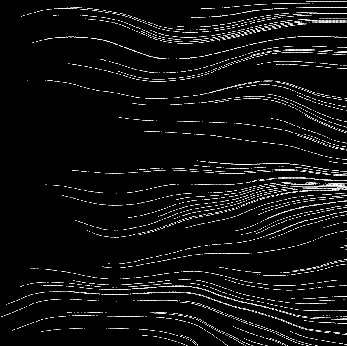
Now our result looks something like this:
That’s looking a bit more interesting! Since the direction of movement of a particle is based solely on the x and y coordinates of the particles position, they tend to converge; if two lines touch each other, they merge into a single line. This looks a bit like what you might see if you looked straight down on a mountain range and looked specifically at rivers and streams on those mountains. Streams near each other are likely on the same side of a slope. They tend to converge into fewer streams.
We are using 2-dimensional noise here. We can add some variation to this pattern by using 3-dimensional noise, with the third dimension being time. Really, we’ll use a counter of the number of frames that have elapsed, or to look at it another way, the number of times the update() and view() functions have been run. Nannou has a function call we can make to get this value. Now update() looks like this:
fn update(app: &App, model: &mut Model, _update: Update) {
    let t = app.elapsed_frames() as f64 / 5000.;
    for i in 0..model.particles.len() {
        let particle = &mut model.particles[i];
        let direction = 10. * model.noise.get([particle.position[0] as f64 / 400., particle.position[1] as f64 / 400., t]);
        particle.update(direction);
    }
}
We are dividing that count by 5000 before using it, so we are getting a fairly small variation. Using a smaller number here will result in a much larger change over time.
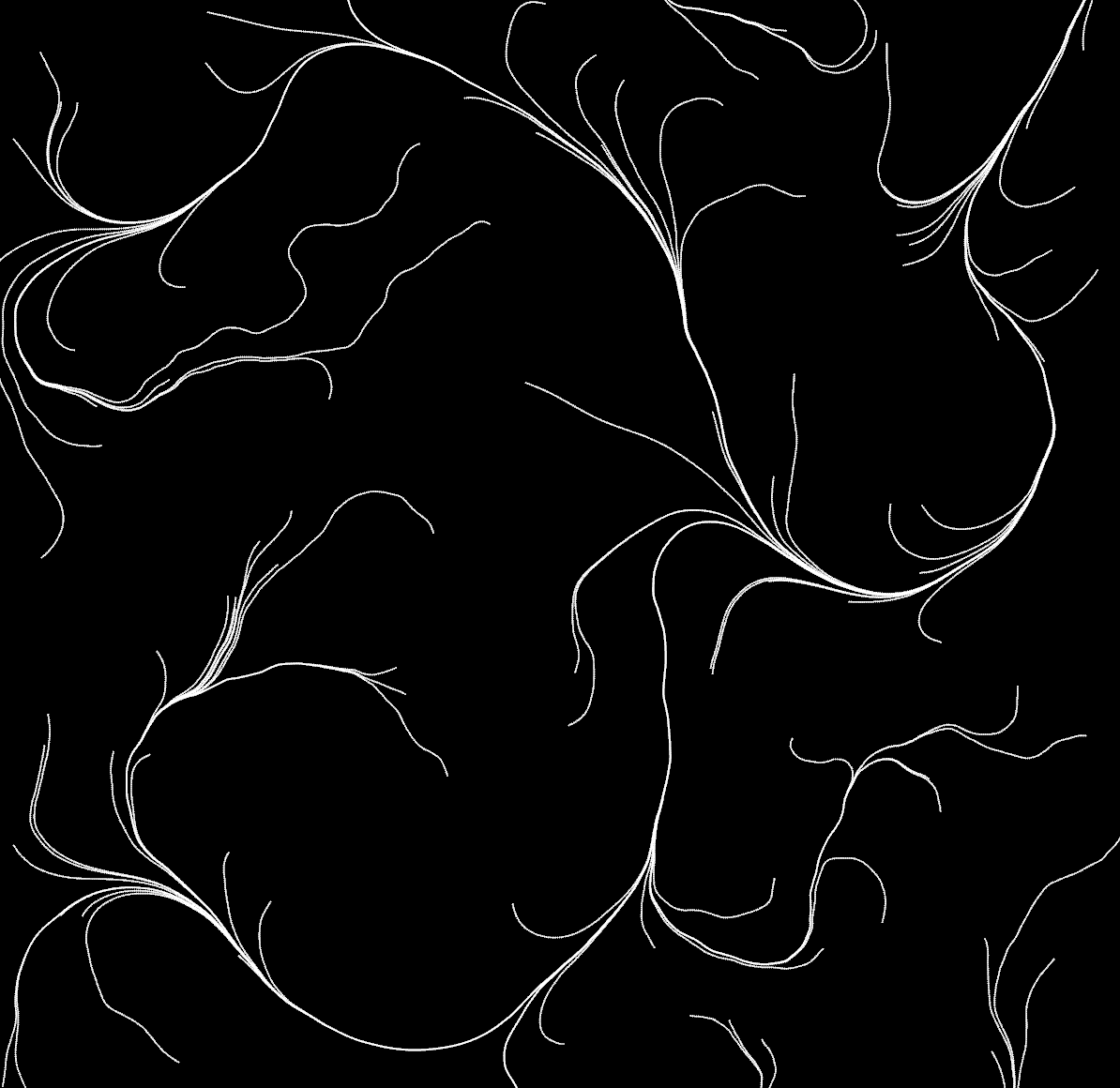
The effect of this will be that if two lines intersect at the same time, they will still converge. But if a line touches another already-existing line, they may not converge. The greater the time between one line touching a point and another line touching the same point, the greater the chance the lines will not converge. There will even be times when they will diverge instead.
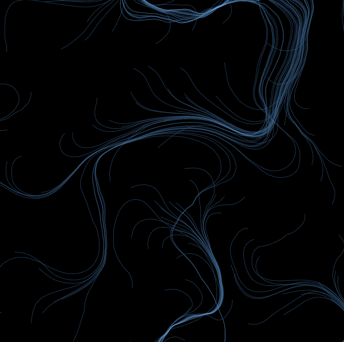
With this change, we now get an image like this one:
Now, those bright white lines are a bit too in-your-face. How can we add some subtlety and color to this? There are many ways to specify color; the one we will use is HSLA (Hue, Saturation, Lightness, Alpha). The hue is the actual color, as a number between 0 and 1. Picture the range from 0 to 1 the same as 0 to 360 degrees on a color wheel. Saturation is how intense the color is, and Lightness is how much light to give the color. Alpha is the transparency of the color. Let’s start by setting the hue, saturation and lightness to some pleasing color, and set the alpha to make it very transparent. The transparency will have the effect of making the lines barely visible, but where lines converge, they will get brighter. We’ll make this change to the view() function:
draw.ellipse().xy(particle.position).w_h(1., 1.).hsla(0.1, 1., 5., 0.01);
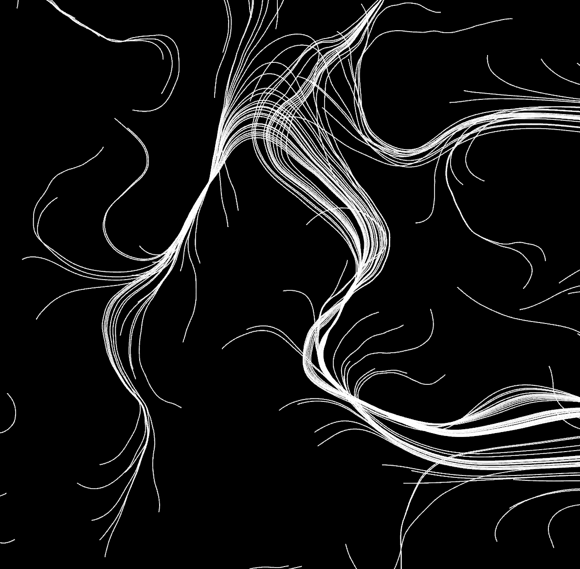
Here is our image now:
Nice, but still boring. If we increase the convergence of the lines by reducing the effect of time (divide the elapsed frames by 50000 instead of 5000) and increase the initial number of points from 100 to 1000, we get an interesting effect:
Lastly, we’ll fuss a little more with the other color parameters. In the view() function, we can vary the colors over time in the same way we did in the update() function:
fn view(app: &App, model: &Model, frame: Frame) {
    let rect = app.window_rect();
    let draw = app.draw();

    let t = (app.elapsed_frames() as f32) / 10000.;
    for particle in &model.particles {
        draw.ellipse().xy(particle.position).w_h(1., 1.).hsla(0.1 + t.sin(), 1. + t / 10000., 5., 0.01);
    }

    draw.to_frame(app, &frame).unwrap();
}
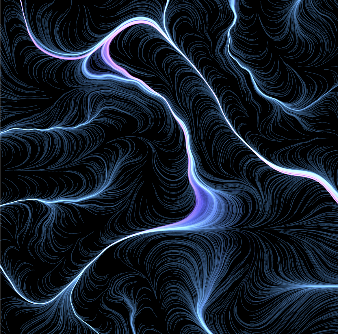
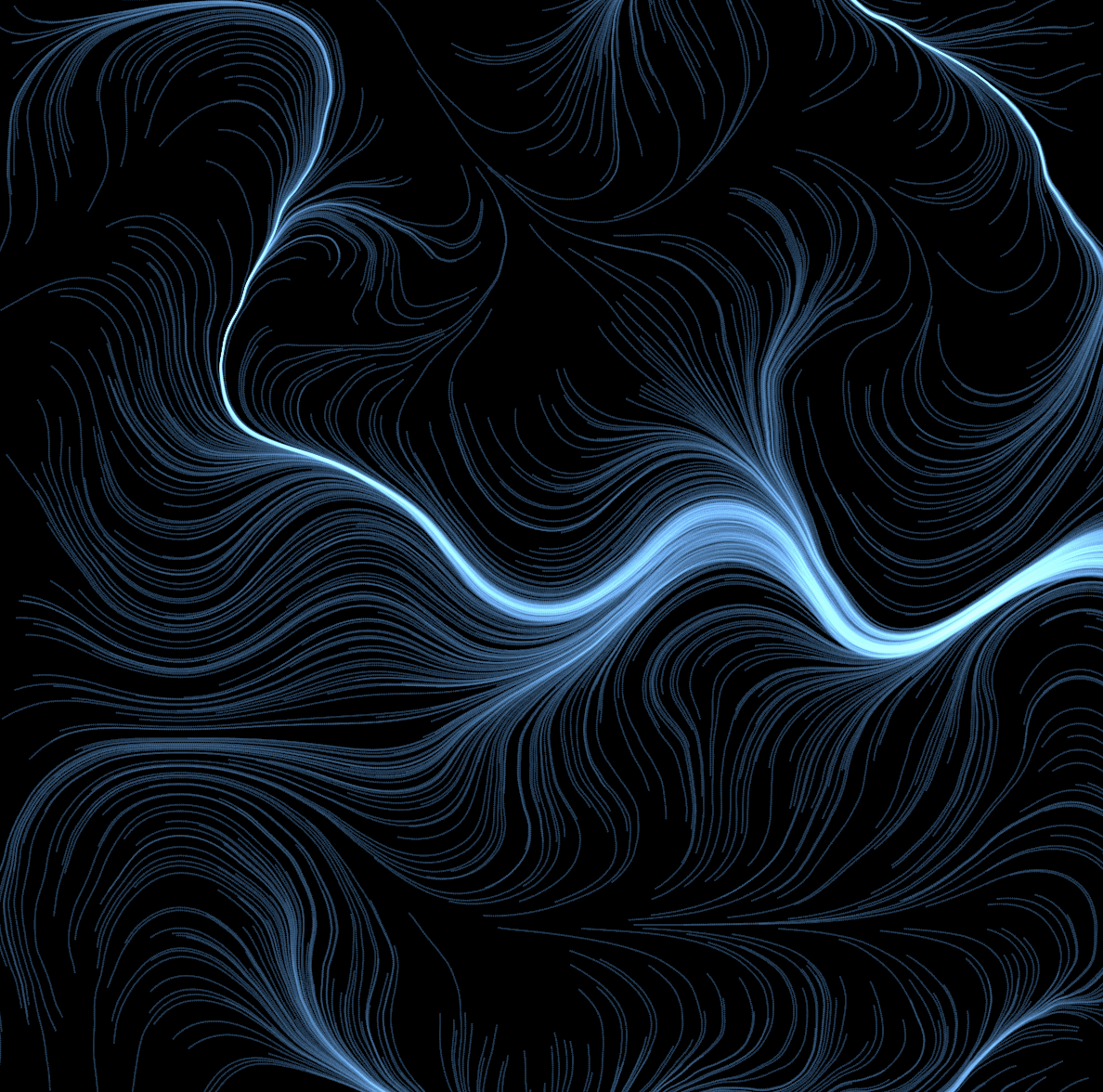
We’ll also increase the number of starting points from 1000 to 3000. Our final image has lots of activity and a bit more color.
You can see the final version of this Nannou app at https://gitlab.com/theartistshusband/noise/-/blob/main/streams/src/main.rs.
Hopefully, this demonstration showed you some ways to use noise to apply randomness to your art in a more controlled, consistent manner, and gave you some ideas to explore!