In my last post , I talked about generative art, and showed a simple example using Javascript and the p5.js library. In this post, I’ll show another relatively simple example using slightly different techniques. Basically, the process is still the same: program the computer to generate a simple drawing and add an element of randomness. For this example, I am still using Javascript and p5.js.
Many of you may be unfamiliar with Javascript. In this post, I am using Javascript, and am trying to make it as clear as possible. But I am not trying to teach you Javascript. If you would like to learn more about Javascript or programming in general, there are some excellent on-line resources, some free, some not. Javascript is not the only programming language that could be used, I chose it for this series of posts because it’s probably the easiest to get started with (open the online editor in your browser and just start adding code!) If you are already familiar with another language, there is a good chance you can find a way to do art with it!
Globular Cluster
In Drunken Lines , we just drew random, connected lines snd let the progran run until it looked interesting. For this example, we’ll generate all the random points up from and come up with interesting ways to display them.
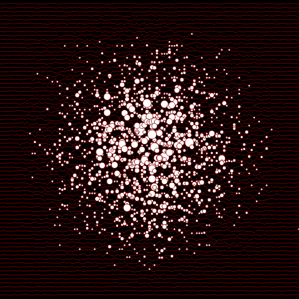
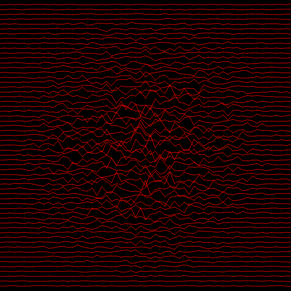
The image at the top of this post is called Globular Cluster. It wasn’t what I had in mind when I started this project, but when I completed what I did have in mind, it was kind of boring, so I took it a step further, and I rather like the result.
The Lines
At the core of this image is a grid of points, spread out more or less evenly. It’s the randommess that causes them to be less even. To start with, we’ll just generate and display a list of points connected with lines. Here is the Javascript code:
const height = 600;
const width = 600;
const xIncr = 10;
const yIncr = 10;

let rows = [];

function setup() {
    createCanvas(width, height);
    background(220);
    stroke(0, 0, 0);

    let y = yIncr;
    while (y < height) {
        let x = 0;
        let row = [{x: x, y: y}];
        while (x < width) {
            x += xIncr;
            row.push({x: x, y: y});
        }
        rows.push(row);
        y += yIncr;
    }
}

function draw() {
    for (let r=0; r<rows.length; r++) {
        for (let c=1; c<rows[r].length; c++) {
            line(rows[r][c-1]['x'], rows[r][c-1]['y'], rows[r][c]['x'], rows[r][c]['y']);
        }
    }

    noLoop();
}
First we define height and width as the size of the canvas we want to draw on, and xIncr and yIncr as the spacing for the points. So we will have a point at every 10th pixel. The rows variable is an array, a list of similar items. In this case, there will be one element in the array for each horizontal row of point. Each element of this array will itself be another array that will be the list of all the points in that row. The points in the array look like this:
{
    x: 10,
    y: 15,
}
This is an object containing two items, x and y, which are both numbers. This example is an object the describes the point (10,15).
You may remember from my previous post that there are two basic functions in p5.js: setup() and draw(). The setup() function runs once, and the draw() function runs continuously until you end the program or tell the function to stop. In the example above, we are creating the canvas and building the list of points in the setup() function. We do this with two while loops. First we set y to yIncr, which in this example is 10. We start here instead of at 0 because we don’t want a line at the very top of the canvas. Then while y is less than height, we build the list of points on that line, add yIncr to y, and go back to the top of the loop. Once y becomes greater than height, the loop ends.
Inside the y < height loop is where we generate all the values of x for that value of y. First we set x to 0. Unlike y, we do want x to start at 0, the edge of the canvas. Then we create the row array with the first point, which will be (0, y). We use a while loop to generate these points. This is very much like the first loop, but runs while x, which we started at 0, is less than width. There is a subtle difference here. In the y < height loop, we run the x < width loop, then we increment y at the end of the loop. When it loops back to the top, we test y, and if it is greater than height, we stop looping. This means that the last value of y will always be on the canvas – if the next value of y is off the canvas, we stop. Inside the x < width loop, however, we increment x at the top of the loop, then generate the point (the row.push({x: x, y: y}); statement add a new point to the row array.) That means x was inside the canvas when we started, but then we increment it, so the value of x for the last point will always be somewhere to the right of the canvas. Why? Remember that we started x at 0, but put the first point in the row before starting the loop. So when we enter the loop, x is already the value of the last point in the row – the first thing we have to do is increment x. It’s not a problem that the last point is always off the canvas because we intend to use these points to draw a line through each row. This way our line will always go edge-to-edge on the canvas.
But why create the first point before the x < width loop? Why not just use the loop to create all the points? We certainly could have done that! But later we are going to change the value of y inside the loop to create interesting patterns. By making sure the first point on each row has the original value of ‘y’, we can use it in some calculations. We’ll do that later in this post.
The setup() function creates all the points, but the draw() function actually displays them. Remember that the rows array is a list of all the rows. Each row is an array that is a list of all the points in a row. And each point is an object with an x value and a y value. The first element in each array is element 0. So for example the 4th row is accessed as:
rows[3]
The 3rd point in the 4th row is:
rows[3][2]
And the x and y values in that point are:
rows[3][2]['x']
rows[3][2]['y']
We want to draw lines from each point to the next on each row, so we’ll se a for loop to look at each element in the rows from 0 to the last one’. Inside that loop, we’ll do another for loop over the list of points in the that row, from 1 to the last one. Why from 1 and not from 0? Because in each case, were going to draw a line from the previous point to the current point, and point 0 doesn’t have a previous point.
Inside the second loop, we have the row number r, and the column number c, we can use those values to get to the current point, and by subtracting 1 from c, the previous point in the row. So we can draw a line like this:
line(rows[r][c-1]['x'], rows[r][c-1]['y'], rows[r][c]['x'], rows[r][c]['y']);
For example, if we are looking at the 3rd point in the 4th row, rows[3][2], r is 3 and c is 2. So we’ll draw a line from the point in rows[3][1] to the one in rows[3][2]. The actual coordinates for that point on the canvas are stored in the point object.
After all the lines are drawn, the draw() function runs the noLoop() function. Remember that the draw function runs over and over forever (well, until the program is stopped), and noLoop() tells it not to do that – so draw() only runs once. This is fine, because it only takes once to draw all our lines.
This is the image the above program builds.

It’s a bit boring, just a bunch of horizontal lines, 10 pixels apart. Each line is really just a bunch of shorter lines, each 10 pixels long, laid end to end, but you can’t really tell that from the image. Let’s improve on that some!
Line Variations
On each row, lets vary the value of y slightly for each line. To do this we’ll modify the y value slightly for each point as we create it in the setup() function. We’ll add a function called modifyY(), and we’ll pass it both x and y for each point. It will pass back a new value for y. Why pass it x? We won’t use it in this first example, but we will be using it later on so that we can change y differently depending on where the point is in the row.
This is the new function:
function modifyY(x, y) {
  let newY = y + Math.floor(random(-yIncr, yIncr+1))

  return newY;
}
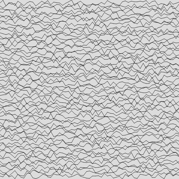
This function generates a random number between -yIncr and yIncr, adds it to the original y and returns it. Since yIncr is set to 10, y will vary randomly by as much as 10.
To use this new value, call this function when generating each point in setup() instead of just using the original y.
row.push({x: x, y: modifyY(x, y)});
Now our image looks like this:
Let’s change the modifyY() function so that y varies more in the center of the image.
function modifyY(x, y) {

    let maxEntropy = {
        x: width/2,
        radiusX: width/2,
    };
    let entropyX = Math.max((maxEntropy['radiusX'] - Math.abs(x - maxEntropy['x'])) / maxEntropy['radiusX'], 0);

    let newY = y + Math.floor(randomGaussian(0, yIncr * entropyX));

    return newY;
}
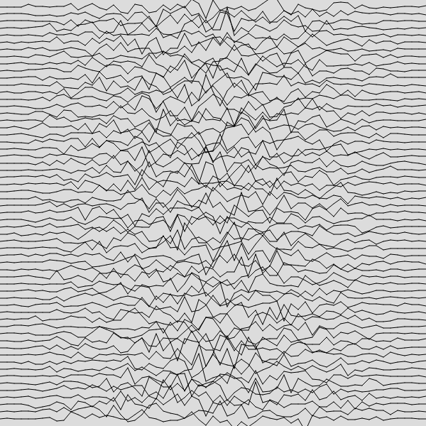
We are declaring a maxEntropy object with some information we’ll need for the calculation. maxEntropy['x'] is where in the row we want y to vary the most, and of course width/2 is the vertical center of the image. maxEntropy['radiusX'] affects how wide the area of variation should be. Since it is also set to width/2, we should have y varying very little for the first and last parts of each row, and much more for the middle. This will not be exact, and there will be a gradual transition, not a sharp division.
We will use a different randomizing function this time: randomGaussian(). With random(), you give it a range of numbers, and you get back a random number somewhere in that range, with the probability of all numbers in that range being the same. With randomGaussian(), you pass in a mean (average) and a standard deviation.
The Standard Deviation is a measure of the dispersion of a set of values. A lower standard deviation means that the values tend to be close to the center value, or mean. A higher standard deviation means that the values are more spread out. For a standard deviation of σ, about 68% of the valies will be no more than σ from the mean, about 95% will be no more than 2σ from the mean, and about 99.6% will be within 3σ from the mean.
randomGaussian() could return pretty much any number, but the changes of it returning anything more than 3 times the standard deviation from the mean are quite small.
In modifyY(), we are calculating entropyX, which will be the amount of variation we want in y based on the value of x. That’s rather scary looking, so I’ll break it down.
Math.abs(x - maxEntropy['x']))
This is the distance of x, in pixels, from maxEntropy['x']. The closer to maxEntropy['x'] x is the smaller this value will be. But we want a value that is greatest at maxEntropy['x'], so let’s convert it to a range from 1 when we are right on maxEntropy['x'] to 0 when we are more than maxEntropy['radiusX'] away from `maxEntropy[‘x’].
(maxEntropy['radiusX'] - Math.abs(x - maxEntropy['x']) / maxEntropy['radiusX']
That doesn’t quite work, since if x is more than maxEntropy['radiusX'] away from maxEntropy['x'], then this value is negative.
Math.max((maxEntropy['radiusX'] - Math.abs(x - maxEntropy['x'])) / maxEntropy['radiusX'], 0);
This prevents the value from going below 0, giving us a value between 0 and 1. We multiply this by yIncr to get the standard deviation to pass to randomGaussian(). Why yIncr and not some other value? You can use any value you want, and what you choose will really depend on how pleasing you find the results. For example, if you could multiply the standard deviation by 2, randomGaussian(0, 2 * yIncr * entropyX), and cause the peaks in your final image to be roughly twice as far from the original y.
Now our image looks like this:
Let’s do the same in the vertical direction so we can set a more-or-less spherical area of greatest variation.
function modifyY(x, y) {
    let maxEntropy = {
        x: width/2,
        y: height/2,
        radiusX: width/2,
        radiusY: height/2,
    };
    let entropyX = Math.max((maxEntropy['radiusX'] - Math.abs(x - maxEntropy['x'])) / maxEntropy['radiusX'], 0);
    let entropyY = Math.max((maxEntropy['radiusY'] - Math.abs(y - maxEntropy['y'])) / maxEntropy['radiusY'], 0);
    let entropy = entropyX * entropyY;

    let newY = y + Math.floor(randomGaussian(0, yIncr * entropy));

    return newY;
}
Here we have used the same technique for generating entropyY as we did for entropyX. Since both are random values between 0 and 1, multiplying them together gives another value that us still between 0 and 1. We can use that to generate the standard deviation.
Now our image looks like this.
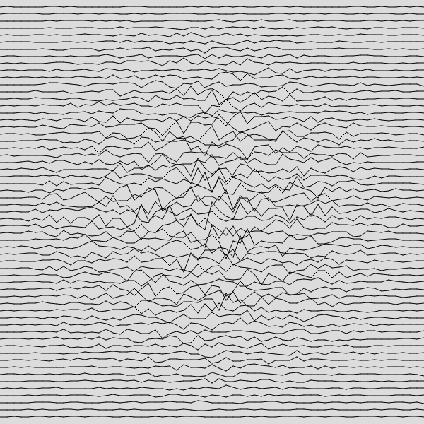
That is what I originally set out to create, but I think it’s fairly boring. So let’s spice it up!
There are 2 lines in the setup() function that set the colors:
background(220);
stroke(0, 0, 0);
These set the background to light grey, and the lines being drawn to black. Instead, lets set the background to black and the lines to red:
background(0);
stroke(255, 0, 0);
Now our image looks like this
The Circles
The last step in creating the Globular Cluster image is to add the circles. These don’t replace the lines, but a drawn on top of them. We’ll draw all the lines first, then the circles, so we just need to add the circle-drawing code to draw(). Here is the new function:
function draw() {
    for (let r=0; r<rows.length; r++) {
        for (c=1; c<rows[r].length; c++) {
            line(rows[r][c-1]['x'], rows[r][c-1]['y'], rows[r][c]['x'], rows[r][c]['y']);
        }
    }
    for (let r=0; r<rows.length; r++) {
        for (let c=0; c<rows[r].length; c++) {
            let diameter = Math.abs(rows[r][0]['y']-rows[r][c]['y']);
            if(diameter > 3) {
                circle(rows[r][c]['x'], rows[r][c]['y'], diameter);
            }
        }
    }

    noLoop();
}
As you can see, we are just cycling through the points again and this time drawing a circle using the p5.js circle() function. This function takes 3 numbers, an x and y location, and a diameter in pixels. We’ll use the x and y values of the point to place the circle, the trick is in calculating the diameter. We’d like diameter of each circle to be the amount that the y value differs from the original y value for that point. Remember that we did not change the value of y for the first point in every row. We can get to that value to figure out much any individual point has changed! So we can calculate the diameter like this:
let diameter = Math.abs(rows[r][0]['y']-rows[r][c]['y']);
That subtracts the current value from the original value, and takes its absolute value because the result could be negative.
To avoid too many very tiny circles, we avoid drawing any with a diameter less than 3.
Now our image looks like this:
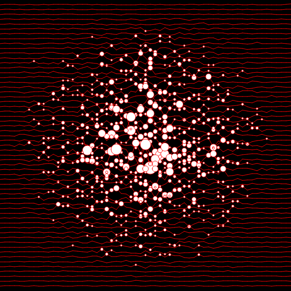
That’s very close to the image at the top of the post! The remaining differences have to do with different values of xIncr and yIncr.
Playing With The Program
This is our ‘final’ program:
const height = 600;
const width = 600;
const xIncr = 10;
const yIncr = 10;

let rows = [];

function setup() {
    createCanvas(width, height);
    background(0);
    stroke(255, 0, 0);

    let y = yIncr;
    while (y < height) {
        let x = 0;
        let row = [{x: x, y: y}];
        while (x < width) {
            x += xIncr;
            row.push({x: x, y: modifyY(x, y)});
        }
        rows.push(row);
        y += yIncr;
    }
}

function draw() {
    for (let r=0; r<rows.length; r++) {
        for (c=1; c<rows[r].length; c++) {
            line(rows[r][c-1]['x'], rows[r][c-1]['y'], rows[r][c]['x'], rows[r][c]['y']);
        }
    }
    for (let r=0; r<rows.length; r++) {
        for (let c=0; c<rows[r].length; c++) {
            let diameter = Math.abs(rows[r][0]['y']-rows[r][c]['y']);
            if(diameter > 3) {
                circle(rows[r][c]['x'], rows[r][c]['y'], diameter);
            }
        }
    }

    noLoop();
}


function modifyY(x, y) {
    let maxEntropy = {
        x: width/2,
        y: height/2,
        radiusX: width/2,
        radiusY: height/2,
    };
    let entropyX = Math.max((maxEntropy['radiusX'] - Math.abs(x - maxEntropy['x'])) / maxEntropy['radiusX'], 0);
    let entropyY = Math.max((maxEntropy['radiusY'] - Math.abs(y - maxEntropy['y'])) / maxEntropy['radiusY'], 0);
    let entropy = entropyX * entropyY;

    let newY = y + Math.floor(randomGaussian(0, yIncr * entropy));

    return newY;
}
It’s really only as final as you want it to be. There is quite a bit that can be done to affect how this looks.
-
Change the
widthandheightof the final image. -
Change
xIncrandyIncrto affect line spacing. -
Change the value of the standard deviations to increase of decrease the variations.
-
Change
maxEntropy['x']andmaxEntropy['y']to center the maximum variation somewhere else on the image, or changemaxEntropy['radiusX']andmaxEntropy['radiusY']to change the size of the area of maximum variation. Make the x and y portions different from each other to affect the shape of the area. Or come up with a different algorithm entirely that changes where the variations appear. -
Use the
stroke()andbackground()functions to modify the colors. These can be called while drawing, so the color can be modified for each point. There is also afill()function which changes the color the circles (and other shapes) are filled in with. We didn’t use it, as the default is white. -
Draw different shapes! p5.js has many to choose from .
-
Draw the lines vertically, in a spiral, in some other order, or just leave them off altogether.
-
Ignore everything I said and do something else entirely!
I have just scratched the surface of the p5.js library. Check out the p5.js web pages for additional instructions and lots of examples .
Have fun!